
Motivation
Last Friday at Red Hat we have another “Day of Learning”, the third one now. As will all repeated things, as an engineer I want to automate things – so this time I wanted to look into machine learning 😉. This was also an excuse to finally learn about NumPy, as that’s such a generic and powerful tool to have on one’s belt.
At school in my 11th grade, I worked on speaker dependent single word speech recognition as my scientific project. This “just” used non-linear time adaption, aka. dynamic programming, to match speech patterns to previously recorded patterns.
23 years later, both the science and the computing power have advanced by leaps and bounds – these days, the go-to solution for such problems are artificial neural networks (called “NN” henceforth), and the “hello world” of that is to recognize handwritten digits. Doing that was my goal.
All the code and notes are in a git repository, and the commits correspond to the various steps that I did.
Admittedly I didn’t manage all of it just on Friday, but it stretched over much of the (fortunately rainy) weekend as well – but it was really worth it!
Prerequisite: NumPy
NNs require a lot of number crunching, but at the same time I really want to think about this problem in mathematical terms like matrix multiplication, not “now I need to allocate 100 bytes for this vector”. NumPy is just for that, so I ran through its quickstart tutorial to lay the basis for notation and computation. After that, manipulating and plotting multi-dimensional arrays looks quite straightforward:
import numpy as np
import matplotlib.pyplot as plt
grad = np.linspace(0,1,10000).reshape(100,100)
plt.imshow(grad, cmap='gray')
plt.show()
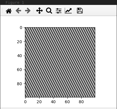
plt.imshow(np.sin(np.linspace(0,10000,10000)).reshape(100,100) ** 2, cmap='gray')
plt.show(block=False)
plt.close()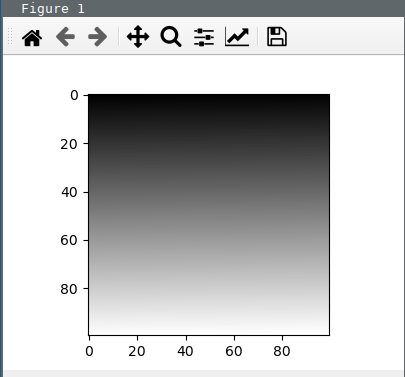
Prerequisite: Annotated data
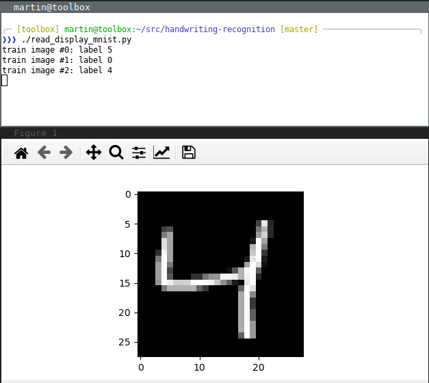
Unlike with my school project’s speech recognizer, which just needed two or three train patterns (in exchange for carefully hand-crafted code), NNs need a lot of training data. Fortunately there is the MNIST database of handwritten digits which is freely available for such purposes. In particular, this has 60,000 labelled images for training and another 10,000 for testing.
Whipping up a parser to turn these databases into NumPy arrays was easy enough, and the read_display_mnist.py script proves that it interprets it correctly:
./download-mnist.sh
NN theory
The internet is full of material about NNs. I stuck to the classic multi-layer feed-forward network with backpropagation training, which somewhat represents the state of the art of 30 years ago, but hey – they are easy to understand and code from scratch. So I started with watching 3Blue1Brown’s excellent video series about the subject. This takes a bit over an hour (with pauses to ponder and take notes), but if you don’t know NNs at all, it is well worth it! Of course Wikipedia also has lots of articles about neurons, perceptrons, backpropagation, etc., which are a nice reference while working on the subject – but at least for me they were too hard to truly grasp as “first-time” material.
One of the best articles that I found was Rafay Khan’s “Understanding & Creating Neural Networks with Computational Graphs from Scratch” which gives both the theory and also working NumPy example code.
Let’s write some Python 🔨
Time to fire up vim and get coding! I started with defining a structure to represent a NN with hidden layers with parametrizable size, and initializing weights and biases randomly. This gives totally random classifications of course, but at least makes sure that the data structures and computations work. I also added add a function test() to recognize the test images and count correct ones. Without training, 10% of the samples are expected to be right by pure chance, and that’s what I get:
$ ./train.py
output vector of first image: [    0.         52766.88424917     0.             0.
 14840.28619491 14164.62850135     0.          7011.882333
     0.         46979.62976127]
classification of first image: 1 with confidence 52766.88424917019; real label 5
correctly recognized images after initialization: 10.076666666666668%
The real fun begins with training, i.e. implementing backpropagation. My first naïve version makes it at least measurably better than the random choice from above, but it is really slow:
$ time ./train.py
[...]
correctly recognized images after initialization: 10.076666666666668%
round #0 of learning...
./train.py:18: RuntimeWarning: overflow encountered in exp
  return 1 / (1 + np.exp(-x))
correctly recognized images: 14.211666666666666%

real	0m37.927s
user	1m19.103s
sys	1m10.169s
This is just one round of training, and usually one needs to do hundreds or even thousands of rounds.
We need moar power! 💪
So I rewrote the code to harness the power of numpy by doing the computations for lots of images in parallel, instead of spending a lot of time in Python on iterating over tens of thousands of examples. And oh my – now the accuracy computation takes only negligible time instead of 6 seconds, and each round of training takes less than a second. This is now with 100 training rounds:
$ time ./train.py
[...]
cost after training round 0: 1.0462266880961681
[...]
cost after training round 99: 0.4499245817840479
correctly recognized images after training: 11.35%

real	1m51.520s
user	4m23.863s
sys	2m31.686s
Tweak time
This is stil rather dissatisfying – even after a hundred training rounds, the accuracy is just marginally better than the 10% random baseline. That’s now the time when you can dial lots of knobs: the size and number of hidden layers, change the initialization of weights, use different activation functions, and so on. But with such a bad performance, the network structure is clearly inappropriate for the task. Apparently, having only 16 neurons in the first hidden layer makes the network not able to “see enough details” in the input. So I changed it to use 80 neurons in the first hidden layer, and drop the second layer (it only seems to make things worse for me). Naturally a single training round takes much longer now, but after only 20 learning iterations it’s already quite respectable:
$ time ./train.py
correctly recognized images after initialization: 9.8%
cost after training round 0: 0.44906826150516255
[...]
cost after training round 19: 0.13264512640861717
correctly recognized images after training: 89.17%

real	0m47.603s
user	2m12.141s
And after 100 iterations, the accuracy improves even more, and the classification of the first test image looks reasonable:
cost after training round 99: 0.043068345296584126
correctly recognized images after training: 92.86%

output vector of first image: [0.02702985 0.01105217 0.02937533 0.05137719 0.01302609 0.00517254
 0.00360999 0.96093954 0.00806618 0.05078305]
classification of first image: 7 with confidence 0.9609395381131477; real label 7

real	4m10.904s
user	11m21.203s
I also tried to replace the Sigmoid activation function with reLU, which is said to perform better. As that does not bound the output to the interval [0, 1], I saw that my previous learning rate of 1 leads to “overshooting” in the gradient descent, and the cost function actually increased during the learning steps several times; the overall result was much worse. Changing the learning rate to linearly fall during the training rounds helps. But in the end, the result is still a bit worse:
cost after training round 99: 0.07241763398153217
correctly recognized images after training: 92.46%
output vector of first image: [0.         0.         0.         0.         0.         0.
 0.         0.89541759 0.         0.        ]
classification of first image: 7 with confidence 0.8954175907939048; real label 7
I’m completely sure that I’m missing something here and don’t use reLU correctly – but I did not take time any more to dig into that.
I also experimented a bit with Stochastic Gradient Descent to make the learning faster, but curiously I didn’t get much speedup out of that: Large matrix multiplications in NumPy are optimized so crazily hard that the overhead of running more iterations and array split-ups in Python seems to eat up all the speed-up from using test data mini-batches.
With 128 instead of 80 neurons in the hidden layer, sigmoid, and 100 rounds of learning I got an accuracy of 94.17%, which I deem good enough for my “hello world” excursion.
Like in so many cases, an xkcd comic says more than a thousand words – it’s quite hilarious how accurate this is!
